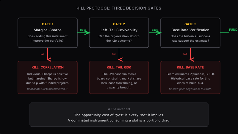
Stop ranking projects. Start killing dominated ones and reallocating the slot.
Three gates in cheapest-first order - marginal Sharpe, left-tail survivability, base rate - decide which instrument loses its funding line so a higher-Sharpe one can have it.
The most important allocator skill is saying no. When your instrument set is large and your capacity is finite, what you don't fund matters more than what you fund. Every slot consumed by a dominated instrument is a slot unavailable for a superior one. The opportunity cost of “yes” is every “no” it implies.
Click a gate to pair it with its kill type.
The Problem
Organizations are bad at stopping. They're reasonably good at starting - there is political energy behind new projects, stakeholder enthusiasm, executive sponsorship. But once a project is funded, three forces conspire to keep it alive past the point where portfolio math says to kill it.
Sunk cost - the money already spent becomes an argument for continuing, even though it is irrelevant to the forward-looking return distribution. The correct question is rarely “how much have we invested?” It is typically “what is the marginal return of the next dollar compared to the strongest alternative use of that dollar (the opportunity-cost benchmark)?”
Political capital - a VP sponsored this project. Killing it feels like a personal rebuke. So the project survives on relationship management rather than return analysis.
Momentum - the team is already staffed. The sprint is already planned. Killing it creates reallocation friction. So the project continues because continuing is the path of least organizational resistance.
Three Kill Types
Not all kills look the same. The instrument being killed may have positive expected value - that is what makes the decision hard. The kill is justified not because the instrument is bad, but because the portfolio is better without it.
1. Correlation-Dominated
The instrument has a positive Sharpe ratio in isolation. But it correlates heavily with something already in the portfolio. The marginal Sharpe of adding it is low - the diversification benefit is near zero.
Consider two builds sharing the same team, the same infrastructure dependency, and the same seasonal timing. The individual Sharpe of each looks attractive. But funding both gives you one concentrated bet with two names, not two independent bets. A third project with lower individual Sharpe but zero correlation produces a better portfolio.
Test: compute the marginal Sharpe after accounting for correlation with existing portfolio. If it drops below the threshold, the slot is better allocated to an uncorrelated alternative.
2. Tail-Risk Violation
The expected value is positive. The -2 sigma case violates a hard constraint. A pricing change that boosts EBITDA in the expected case but risks customer attrition at the left tail hits a market share constraint. The board is telling you: the downside scenario is unacceptable, regardless of the upside.
Left-tail constraints come in three flavors: market share protection (“we cannot lose share in the current period”), timing requirements (“we need cash flow by Q3”), and capacity limits (“we can only run N simultaneous builds”). These are not preferences. They define the feasible region.
Test: for instrument i, is P(R_i < threshold) above the tolerance? If yes, the instrument is outside the feasible set - or it must be paired with a hedge.
3. Base-Rate Overestimation
The team estimates P(success) at 0.8. The historical base rate for this class of build in your organization is 0.3. Two out of seven similar projects reached production and sustained for six months. The team's confidence is not informed by the reference class - it is informed by enthusiasm for this specific project.
When you reprice with the base rate, the Construction Spread goes negative. The instrument looked fundable at the team's estimate. At the organizational base rate, it destroys value.
Example test: pull the historical success rate for comparable builds. If the team's P(success) exceeds the base rate by more than 2x (an illustrative threshold - calibrate to your reference class), require specific evidence for why this project is different from the reference class.
The Decision Sequence
The three gates are sequential because each is progressively more expensive to evaluate. Marginal Sharpe is a spreadsheet calculation. Left-tail analysis requires distribution modeling. Base rate verification requires pulling historical data across comparable projects. Run the cheap gate first.
The Language of No
The hardest part of the kill decision isn't the math. The math is clear. The hard part is the conversation. Telling a VP that their project isn't funded - not because it's bad, but because the portfolio has a better option - requires a vocabulary that “I don't think it's a priority” does not provide.
Portfolio language makes the decision legible. “Your project has an expected return of $300K and a Sharpe of 1.2. But it's correlated 0.7 with Project A. The marginal Sharpe of adding yours is 0.4. Project G has a Sharpe of 3.8 with zero correlation. I'm allocating the slot to G because the portfolio-level return is higher.”
That's an allocator speaking - not a politician, not a prioritizer - but someone constructing a portfolio with explicit math behind every decision. The language does not eliminate the politics. But it shifts the conversation from preference to evidence.
Where AI Fits
AI expanded the instrument set by an order of magnitude. Tasks that had a Templeton Ratio near 1 (no leverage - it takes as long to check as to do) now have T >> 1. The menu of viable investments grew from 5 for 4 slots to 30 for 6 slots. C(5,4) = 5 possible portfolios. C(30,6) = 593,775 possible portfolios.
A larger menu requires more selection discipline, not less. The kill protocol becomes essential when the instrument set expands because the number of dominated instruments grows faster than the number of fundable slots. Without a systematic kill discipline, the portfolio fills with correlated bets, unpriced tail risks, and overestimated success probabilities.
The Automated Kill
Kill decisions also apply to instruments already in execution. The Promotion Protocol encodes this as rollback triggers: if error rate exceeds a threshold, the system demotes automatically. This is a kill decision embedded in the execution layer - no human deliberation required.
The hysteresis gap matters. Promotion at 2% error, rollback at 5%. If the thresholds are equal, the system oscillates. The gap creates a one-way ratchet: hard to promote, easy to sustain, fast to kill on degradation. This is the same asymmetry as the kill protocol - the cost of continuing a bad instrument exceeds the cost of killing a marginal one.
Connection to Other Frameworks
Capital Allocation - the kill protocol is the negative space of portfolio construction. Capital Allocation decides what to fund. Kill Protocol decides what to stop funding.
Promotion Protocol - encodes kill decisions as automated rollback triggers. The execution layer enforces the same portfolio discipline without human deliberation.
Knowledge Capital - instruments that produce no appreciating asset are kill candidates. If the output depreciates (one-off analysis, static reports), the compounding value is zero. Fund the instrument that builds a lasting asset instead.
Construction Spread - the pricing metric that kill decisions act on. A negative spread at base-rate-adjusted P(success) is the quantitative trigger for Kill Type 3.
Automation NPV - models the economics of individual instruments. Kill Protocol uses these models as inputs, then evaluates at the portfolio level.
When kill criteria fail
The protocol rests on a falsifiable claim: killing dominated instruments and reallocating their capacity to higher-Sharpe alternatives raises realized portfolio Sharpe. If this is wrong for an environment, the instruments it declares "dominated" will not underperform relative to the reallocation target. Measure the spread.
The framework does not apply in these cases:
- -Optionality-bearing instruments. When upside distribution (not mean) is the point, Sharpe understates value. Use real-options math, not Sharpe, for pre-product-market-fit bets.
- -Synergy-heavy instruments. Cross-terms between instruments can exceed standalone Sharpe. A dominated-looking instrument may be load-bearing for a higher-value one - score the pair.
- -Strategic or regulatory holds. Some instruments are kept for relationship, option, or compliance reasons at negative expected return. Do not let the protocol kill them; mark them as carried, then apply the protocol to the rest.
- -No reallocation target. If there is literally nothing better to do with the capacity, a dominated instrument beats cash. Kill only when a named replacement is ready to fund.
Rosetta Stone
Four circles, four readings of the same object. Each role reads the artifact through its own lens.
The most important thing the seat does. Allocators say no more than yes. Kill decisions are the proof of discipline; every maintained project represents an implicit re-underwriting.
The mechanism for actually decommissioning a project that's still warm. The protocol is the political cover - "we ran it through the gates" - that lets the team accept the kill without a culture hit.
Deprecation with evidence. The system sunsets because the ratchet said so, not because a VP got bored. Fewer zombie services, cleaner codebase.
A three-stage hypothesis test. Gate 1: marginal Sharpe below threshold. Gate 2: left-tail survivability below threshold. Gate 3: base-rate verification. Failing any gate means reject the continued-investment hypothesis.